Unemployment Claims COVID-19
In this post I am visualizing and analyzing the unprecedented increase in the number of unemployment claims filed in the US after the lockdown due to COVID 19 pandemic. I am retrieving the data from the tidyquant package (Dancho & Vaughan, 2020).
library(CausalImpact)
library(tidyverse)
library(scales)
library(tidyquant)
ICSA Data
Initial unemployment claims from the first date available, 1967:
icsa_dat <- "ICSA" %>%
  tq_get(get = "economic.data",
         from = "1967-01-07") %>%
  rename(claims = price)


glimpse(icsa_dat)
## Rows: 2,790
## Columns: 3
## $ symbol <chr> "ICSA", "ICSA", "ICSA", "ICSA", "ICSA", "ICSA", "ICSA", "ICSA"…
## $ date <date> 1967-01-07, 1967-01-14, 1967-01-21, 1967-01-28, 1967-02-04, 1…
## $ claims <int> 208000, 207000, 217000, 204000, 216000, 229000, 229000, 242000…icsa_dat %>%
ggplot(aes(x = date, y = claims)) +
geom_line(color = "blue") +
scale_y_continuous(labels = comma) +
labs(x = "Date", y = "Claims", subtitle = "As of June 29, 2020") +
ggtitle("Unemployment Claims: 1967 to 2020") +
theme_bw()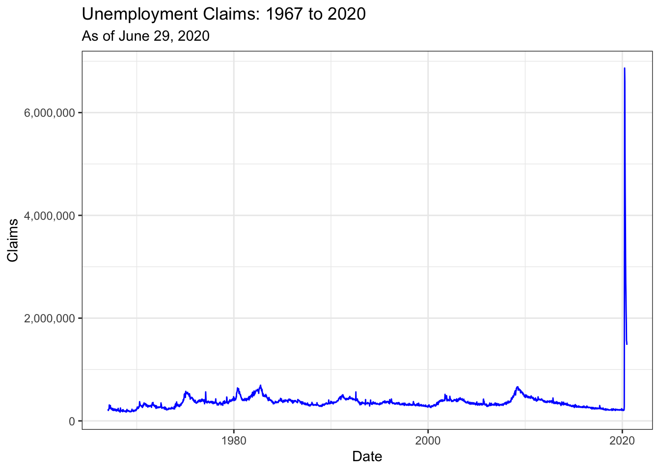
Comparison to 2008 Recession
In the graph below, I only selected 2008 to 2020. We can compare the unemployment claims during the 2008 recession to the number of claims filed during the COVID-19 lockdown. What is happening now is preposterous.
icsa_dat %>%
  mutate(year = year(date)) %>%
  filter(year > 2007) %>%
  ggplot(aes(x = date, y = claims)) +
  geom_line(color = "blue") +
  scale_y_continuous(labels = comma) +
  labs(x = "Date", y = "Claims", subtitle = "As of June 29, 2020") +
  ggtitle("Unemployment Claims: 2008 to 2020") +
  theme_bw()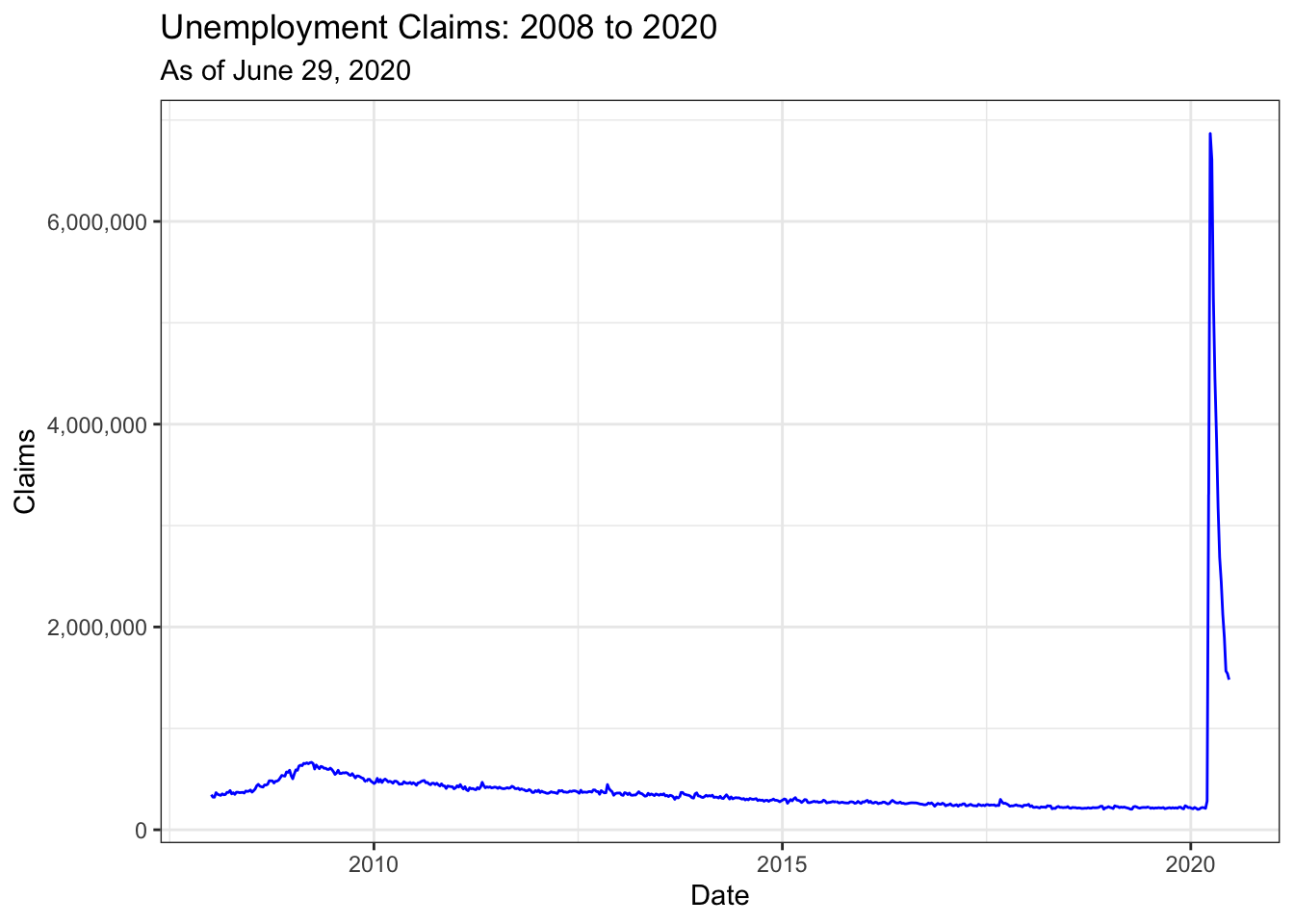
Causal Inference
Sometimes #causalinference is simple.
— Miguel Hernán (@_MiguelHernan) March 29, 2020
“What's the immediate causal effect of the #COVID19 lockdowns on unemployment?”
The answer is “Unprecedented”.
We know we're in deep trouble when a time series is all we need. https://t.co/cXK0wLw3no pic.twitter.com/kS4PvVwihM
Below, I use the CausalImpact package to run a Bayesian structural time-series analysis (Brodersen et al., 2015). For more information on the package, please see this vignette. Typically, it would be good to add covariates in the analysis but the data does not have any and given the rate of increase, I highly doubt that the inclusion of covariates would matter much. It would be interesting to compare the number of claims filed in US versus the number of claims filed in country with better social and economic security systems in place (perhaps the Netherlands). The impact of COVID-19 lockdowns on the number of unemployment claims is probably exacerbated by the lack of social and economic security in the US. In addition, due to employer based healthcare system in the US, millions of people have lost or are going to lose health insurance. Now more than every we need Medicare for All, $2000 a month stimulus, Green New Deal. The impact of climate change will be worse.
Projected⬆️in unemployment:
— Warren Gunnels (@GunnelsWarren) April 21, 2020
🇩🇪: 3.2%➡️5.9%
🇬🇧: 3.9%➡️7%
🇫🇷: 8.5%➡️12%
🇺🇸: 3.5%➡️32.1%
Projected⬆️ in # of uninsured:
🇩🇪: 0
🇬🇧: 0
🇫🇷: 0
🇺🇸: At least 12 million
Solution: Guarantee healthcare and paychecks like other wealthy countries do. https://t.co/44ijS2evzL
dates <- icsa_dat %>%
  pull(date)

# create pre and post
pre_period <- c(dates[1], dates[2776])
post_period <- c(dates[2777], dates[length(dates)])

# make into dat
dat <- icsa_dat %>%
  select(date, y = claims)

# causal impact
impact <- CausalImpact(dat, pre_period, post_period)

sum_impact <- impact$summary %>%
  mutate(type = rownames(.)) %>%
  pivot_longer(cols = -type,
               names_to = "stats",
               values_to = "vals")

avg_impact <- sum_impact %>%
  mutate(vals = round(vals/1000000, 2))

rel_impact <- sum_impact %>%
  filter(str_detect(stats, "Rel")) %>%
  mutate(vals = round(vals * 100))

# summary(impact, "report")
Analysis report: CausalImpact
Below is the report generated by CausalImpact with some edits by me.
Summing up the individual data points during the post-lockdown period, the total number of unemployment claims filed equaled 47.25M. By contrast, had the intervention not taken place, we would have expected a sum of 3.54M. The 95% interval of this prediction is [2.88M, 4.21M].
The probability of obtaining this effect by chance is very small (Bayesian one-sided tail-area probability p = 0.001). This means the causal effect can be considered statistically significant.
References
Brodersen et al., 2015, Annals of Applied Statistics. Inferring causal impact using Bayesian structural time-series models. http://research.google.com/pubs/pub41854.html
Dancho, M. and Vaughan, D. (2020). tidyquant: Tidy Quantitative Financial Analysis. R package version 1.0.0. https://CRAN.R-project.org/package=tidyquant
Wickham, H. and Seidel, D. (2019). scales: Scale Functions for Visualization. R package version 1.1.0. https://CRAN.R-project.org/package=scales
Wickham et al., (2019). Welcome to the tidyverse. Journal of Open Source Software, 4(43), 1686, https://doi.org/10.21105/joss.01686